micropython-nano-gui/FPLOT.md

fplot module

This provides a rudimentary means of displaying two dimensional Cartesian (xy) and polar graphs on framebuf based displays. It is an optional extension to the MicroPython nano-gui library: this should be installed, configured and tested before use.

This was ported from the lcd160cr-gui library. Like nanogui.py it uses synchronous code.

Please excuse the photography: these displays look much better than in my pictures.

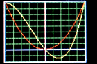Classic Cartesian plot.

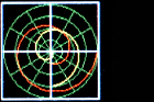
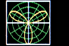Classic polar plot.

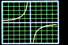Plot of discontinuous data.

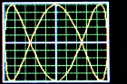A Lissajous figure.

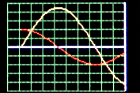Still from a simulation of plotting realtime data using the TSequence class.

Still from a simulation of realtime acquisition of two varying vectors.

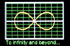The lemniscate of Bernoulli.

Contents

1. Python files
2. Concepts
   2.1 Graph classes
   2.2 Curve clsses
   2.3 Coordinates
3. Graph classes
   3.1 Class CartesianGraph
   3.2 Class PolarGraph
4. Curve classes
   4.1 class Curve
   4.1.1 Scaling Optional scaling of data values.
   4.2 class PolarCurve
   4.2.1 Scaling Required scaling of complex points.
   4.3 class TSequence Plot Y values on time axis.

Main README

1. Python files

These are located in the plot directory.

1. fplot.py The plot library
2. fpt.py Test program. Usage examples.

Before attempting to use this library please install and test the nanogui module on your hardware.

2. Concepts

Data for Cartesian graphs constitutes a sequence of x, y pairs, for polar graphs it is a sequence of complex z values. The module supports three common cases:

1. The dataset to be plotted is complete at the outset.
2. Arbitrary data arrives gradually and needs to be plotted as it arrives.
3. One or more y values arrive gradually. The X axis represents time. This is a simplifying case of 2.

2.1 Graph classes

A user program first instantiates a graph object (PolarGraph or CartesianGraph). This creates an empty graph image upon which one or more curves may be plotted.

2.2 Curve classes

The user program then instantiates one or more curves (Curve or PolarCurve) as appropriate to the graph. Curves may be assigned colors to distinguish them.

A curve is plotted by means of a user defined populate generator. This assigns points to the curve in the order in which they are to be plotted. The curve will be displayed on the graph as a sequence of straight line segments between successive points.

Where it is required to plot realtime data as it arrives, this is achieved via calls to the curve's point method.

2.3 Coordinates

Graph objects are sized and positioned in terms of TFT screen pixel coordinates, with (0, 0) being the top left corner of the display, with x increasing to the right and y increasing downwards. By nanogui convention a border, if specified, extends two pixels beyond the graph in each direction. If the graph is placed at [row, col] the top left hand corner of the border is at [row-2, col-2]. The coordinate system within a graph conforms to normal mathematical conventions.

Scaling is provided on Cartesian curves enabling user defined ranges for x and y values. Points lying outside of the defined range will produce lines which are clipped at the graph boundary.

Points on polar curves are defined as Python complex types and should lie within the unit circle. Points which are out of range may be plotted beyond the unit circle but will be clipped to the rectangular graph boundary.

Contents

3. Graph classes

3.1 Class CartesianGraph

Constructor.
Mandatory positional arguments:

1. writer A CWriter instance.
2. row Position of the graph in screen coordinates.
3. col

Keyword only arguments (all optional):

• height=90 Dimension of the bounding box.
• width=110 Dimension of the bounding box.
• fgcolor=None Color of the axis lines. Defaults to Writer forgeround color.
• bgcolor=None Background color of graph. Defaults to Writer background.
• bdcolor=None Border color. If False no border is displayed. If None a border is shown in the Writer forgeround color. If a color is passed, it is used.
• gridcolor=None Color of grid. Default: Writer forgeround color.
• xdivs=10 Number of divisions (grid lines) on x axis.
• ydivs=10 Number of divisions on y axis.
• xorigin=5 Location of origin in terms of grid divisions.
• yorigin=5 As xorigin. The default of 5, 5 with 10 grid lines on each axis puts the origin at the centre of the graph. Settings of 0, 0 would be used to plot positive values only.

Methods:

1. clear No args. Clears all curves from the graph.
2. show No args. Redraws the graph. For future/subclass use.

3.2 Class PolarGraph

Constructor.
Mandatory positional arguments:

1. writer A CWriter instance.
2. row Position of the graph in screen coordinates.
3. col

Keyword only arguments (all optional):

• height=90 Dimension of the square bounding box.
• fgcolor=None Color of the axis lines. Defaults to Writer forgeround color.
• bgcolor=None Background color of graph. Defaults to Writer background.
• bdcolor=None Border color. If False no border is displayed. If None a border is shown in the Writer forgeround color. If a color is passed, it is used.
• gridcolor=None Color of grid. Default: Writer forgeround color.
• adivs=3 Number of angle divisions per quadrant.
• rdivs=4 Number radius divisions.

Methods:

1. clear No args. Clears all curves from the graph.
2. show No args. Redraws the graph. For future/subclass use.

Contents

4. Curve classes

4.1 class Curve

The Cartesian curve constructor takes the following positional arguments:

Mandatory arguments:

1. graph The CartesianGraph instance.
2. color If None is passed, the graph foreground color is used.

Optional arguments:
3. populate=None A generator to populate the curve. See below.
4. origin=(0,0) 2-tuple containing x and y values for the origin. Provides for an optional shift of the data's origin.
5. excursion=(1,1) 2-tuple containing scaling values for x and y.

Methods:

• point Arguments x, y. Defaults None. Adds a point to the curve. If a prior point exists a line will be drawn between it and the current point. If a point is out of range or if either arg is None no line will be drawn. Passing no args enables discontinuous curves to be plotted. This method is normally used for real time plotting.

The populate generator may take zero or more positional arguments. It should repeatedly yield x, y values before returning. Where a curve is discontinuous None, None may be yielded: this causes the line to stop. It is resumed when the next valid x, y pair is yielded.

If populate is not provided the curve may be plotted by successive calls to the point method. This may be of use where data points are acquired in real time, and realtime plotting is required. See function rt_rect in fpt.py.

4.1.1 Scaling

By default, with symmetrical axes, x and y values are assumed to lie between -1 and +1.

To plot x values from 1000 to 4000 we would set the origin x value to 1000 and the excursion x value to 3000. The excursion values scale the plotted values to fit the corresponding axis.

4.2 class PolarCurve

The constructor takes the following positional arguments:

Mandatory arguments:

1. graph The PolarGraph instance.
2. color

Optional arguments:
3. populate=None A generator to populate the curve. See below.

Methods:

• point Argument z=None. Normally a complex. Adds a point to the curve. If a prior point exists a line will be drawn between it and the current point. If the arg is None no line will be drawn. Passing no args enables discontinuous curves to be plotted. Lines are clipped at the square region bounded by (-1, -1) to (+1, +1).

The populate generator may take zero or more positional arguments. It should yield a complex z value for each point before returning. Where a curve is discontinuous a value of None may be yielded: this causes plotting to stop. It is resumed when the next valid z point is yielded.

If populate is not provided the curve may be plotted by successive calls to the point method. This may be of use where data points are acquired in real time, and realtime plotting is required.

4.2.1 Scaling

Complex points should lie within the unit circle to be drawn within the grid.

Contents

4.3 class TSequence

A common task is the acquisition and plotting of real time data against time, such as hourly temperature and air pressure readings. This class facilitates this. Time is on the x-axis with the most recent data on the right. Older points are plotted to the left until they reach the left hand edge when they are discarded. This is akin to old fashioned pen plotters where the pen was at the rightmost edge (corresponding to time now) with old values scrolling to the left with the time axis in the conventional direction.

The user instantiates a graph with the X origin at the right hand side and then instantiates one or more TSequence objects. As each set of data arrives it is appended to its TSequence using the add method. See the example below.

The constructor takes the following args:

Mandatory arguments:

1. graph The CartesianGraph instance.
2. color
3. size Integer. The number of time samples to be plotted. See below.

Optional arguments:
4. yorigin=0 These args provide scaling of Y axis values as per the Curve class. 5 yexc=1

Method:

1. add Arg v the value to be plotted. This should lie between -1 and +1 unless scaling is applied.

Note that there is little point in setting the size argument to a value greater than the number of X-axis pixels on the graph. It will work but RAM and execution time will be wasted: the constructor instantiates an array of floats of this size.

Each time a data set arrives the graph should be cleared, a data value should be added to each TSequence instance, and the display instance should be refreshed. The following example assumes that ssd is the display device and wri is a Writer or CWriter instance.

def foo():
    refresh(ssd, True)  # Clear any prior image
    g = CartesianGraph(wri, 2, 2, xorigin = 10, fgcolor=WHITE, gridcolor=LIGHTGREEN)
    tsy = TSequence(g, YELLOW, 50)
    tsr = TSequence(g, RED, 50)
    for t in range(100):
        g.clear()
        tsy.add(0.9*math.sin(t/10))
        tsr.add(0.4*math.cos(t/10))
        refresh(ssd)
        utime.sleep_ms(100)

Contents